Non-parametric Bayesian updating
This page explains my work on this topic and is a repository for code and extended outputs that could not fit into publications. The code is ©BayesCamp Ltd 2021-present, and licensed for use CC-BY-4.0. The text and images in this web page are also ©BayesCamp Ltd 2021, except the Wikimedia photograph, and are NOT licensed for reuse (all rights reserved). You may use the code as you wish, as long as you acknowledge the source. I suggest you publicly display this: "Adapted from code by Robert Grant, CC-BY-4.0 (c) BayesCamp Ltd, Winchester, UK". However, you may NOT distribute or publish the rest of this web page in ANY form without the explicit written consent of BayesCamp Ltd. I'm thinking of phony bloggers here. Send requests to email given above in the menu bar. If you find it useful and want to say thanks, you can click on Buy Me A Coffee below and do just that.
Table of Contents
"Year after year
Feeding cherry trees
Blossom fragments"
— Matsuo Basho (1691), trans. Takafumi Saito & William R Nelson
Primer
Bayesian updating is the principle that you can add data sequentially in batches to learn a posterior distribution. If done correctly, the result will be the same as if you had analysed all data together.
In my experience, teachers of intro Bayes courses talk about this all the time. Then it never gets used in real life. Why not?
Teachers lie to you. I know because I am one. We show you some nice, well-behaved, one-parameter examples with conjugate priors and everything looks simple. Well, real life Bayes is harder than that, so let's buckle up. A prior is actually a joint density over all the parameters and other unknowns in your model, even though probabilistic programming languages like BUGS, Stan and PyMC* have drawn us into thinking of it as a series of marginal distributions, one for each parameter. Parameters are generally correlated with each other, so the joint specification cannot be reduced to a set of marginal distributions without loss of the correlation information. Another problem is that multimodality or non-linearity might be masked by the marginal distributions.
Parametric updating is possible if you correctly know the joint distribution. You can specify hyperparameters for the next prior by analysing the previous posterior. In the case of a multivariate normal prior and posterior for p parameters, this would mean a vector of p means and a p-by-p covariance matrix.
But we do not know the distribution. That's why we're doing the analysis.
A non-parametric updating method would use the posterior sample to inform the prior density. In this sense, we have yesterday's posterior sample, and we are going to use it as today's prior sample. Because these samples can have a dual purpose, I call them p[oste]riors.
.jpg)
A winter scene of kudzu growing over bushes and trees at Floyd Bennett Field, New York. Image by wikmedia user "Rhododendrites", CC BY-SA 4.0, via Wikimedia Commons
At heart, this is a density estimation problem. Given the prior sample, we need to be able to obtain a prior density at any proposed parameter vector. I think of this as a surface in p-dimensional parameter space. The classic method is kernel density estimation, but this will not work for anything but the smallest p, maybe p<5. This is long established and I demonstrated it in this context in the IJCEE paper.
Instead, I devised the kudzu algorithm, which uses density estimation trees (DET), a fast and scalable method which uses the same tree-growing algorithm from classification and regression trees, but to estimate a density. The DET estimate is piecewise constant, which will not help with Bayesian sampler algorithms such as Hamiltonian Monte Carlo (implemented in Stan and PyMC*), Metropolis-adjusted Langevin Algorithm or Piecewise Deterministic Markov Processes; these samplers need to obtain and use gradients of the density (the Jacobian vector) and the estimated density should be smooth.
To smooth the DET estimate, I replace the edges of leaves (you might say I "convolve" them) with inverse logistic ramp functions. The formulas and code are below. Evaluation shows kudzu performing with comparable fidelity to kernel density in low-p problems, and performing quickly and accurately in p up to 50. It hasn't been tested past that (yet), but I don't see any reason why it would deteriorate.
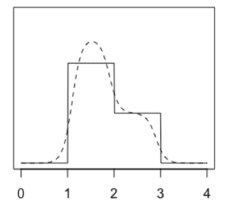
A one-dimensional illustrative set of two leaves (solid lines) and a corresponding kudzu density (dashed curve)
Formulas for the kudzu algorithm
DET returns a collection of leaves, each of which has a top and bottom value in each dimension, and a density. This is like a collection of multivariate uniform densities (which are zero outside the leaf). Imagine the complete DET density estimate as the sum of all these leaves' multivariate uniform densities. We will construct kudzu density in the same way, as a sum of leaves.
The kudzu leaves have uncorrelated multivariate densities, so we can construct those in turn as the product of univariate densities. Each of those univariate densities is the product of two inverse logistic ramps.
Statistically minded readers might get some extra intuition from the fact that the inverse logistic ramp is the logistic distribution's CDF. Its derivative (the logistic PDF) is the product of two inverse logistic ramps sharing a common midpoint (where their ordinate is 0.5), but facing in opposite directions. If we move those two ramps further apart or closer together, and potentially alter their steepness, we have a univariate component for one kudzu leaf.
This is the notation in the formulas:
- θ is a vector of proposed parameter values, evaluated by one iteration of a sampling algorithm
- ℓ is a natural number identifying one leaf of the DET
- fDET(ℓ) is the density estimated by DET for that leaf (a positive real number)
- j is a natural number identifying one of the parameters (one dimension of the distribution)
- μb is the location of the bottom of the leaf in the jth dimension; μt is the top; they share support with θj
- σ is a positive real number, the scaling factor for the steepness of the ramp, a bandwidth controlling the tradeoff between smoothness and detail (also, if sigma gets too big, it will inflate the marginal distributions)
- δb is a distance by which we move the midpoint of the ramp either side of μb, to control variaince inflation; δt is the same for μt; I call this delta-translation
- φ is a positive real number, the number of sigmas on either side of μt+δt and μb+δb, up to which we evaluate the integral
In practice, I found that there has to be delta-translation towards the mode of the density, in order to control variance inflation. Heuristically, I did this in the IJCEE paper by finding the centre of the leaf (hypercuboid) of highest predicted density; this is the approximate mode. Then, each edge of each leaf is moved towards it by delta, times the sine of the angle between the edge and a line joining the centre of that edge to the approximate mode. In this setting, δb=δt.

The inverse logistic function
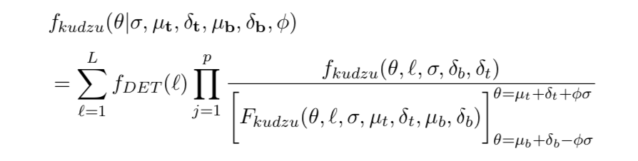
The kudzu density is the sum of the leaves' densities. Each of those is the product of the univariate components, with each one normalised by dividing by its integral. The numerator and denominator are defined below.
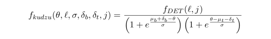
The numerator of the kudzu density in the jth dimension of the ℓth leaf. Because this will not generally integrate to one, it is not a probability density until it has been normalised. fDET(ℓ,j) is the marginal density of the DET density for that leaf in the jth dimension.

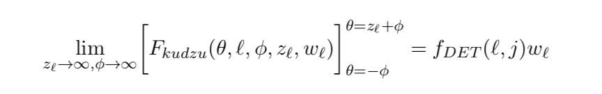
The denominator of the kudzu density in the jth dimension of the ℓth leaf, the definite integral over [μb+δb-φσ, μt+δt+φσ], is equivalent to setting σ=1, μb+δb=0, μt+δt=zℓ, and then evaluating over [-φ, zℓ+φ]. Writing it in this form leads to the limits below.
If a particular dimension of a leaf is wide enough, relative to the bandwidth, to have a plateau in the middle, then the integral simplifies to the area under the rectangle between ramp midpoints. Let wℓ = μt+δt-μb-δb be the width of the leaf, and zℓ = (wℓ)/σ the width in units of σ in the jth dimension. I suggest zℓ>12 as a rough guide.
Two further considerations remain. First, kudzu, being based on orthogonal partitioning of the parameter space, will work best on uncorrelated priors. (Ensembles of kudzu densities may help, see below.) So, I standardise the prior sample by subtracting means and Hadamard-dividing by standard deviations. Then, I apply principal components analysis (PCA) rotation (premultiplication with the eigenvector matrix), and finally I rescale again by Hadamard-division by standard deviations of these rotated variables. Kudzu is applied to this. Inside Stan (or other sampling algorithms), we estimate the prior density using this, then back-transform the proposed parameter vector into the parameters of the likelihood, and evaluate the likelihood.
Secondly, we must apply a small gradient outside the prior sample bounding box (smallest hypercuboid containing all prior draws), in order to guide the sampler back to the region of highest density. I do this by mixing 0.98 times the kudzu density with 0.02 times a multivariate normal density, centred on the approximate mode and with standard deviation twice that of the largest principal component standard deviation.
The denominator of the kudzu density in the jth dimension of the ℓth leaf, if it is wide enough to allow for a plateau and hence no interference between the two ramps.
Software for the kudzu algorithm
Now, in 2024, I have an R package and Stata commands underway. These will start to appear at conferences over the summer, then online here. You will be able to:
- Fit a density estimation tree that supplies output amenable to kudzu
- Optimise the tuning parameters of the kudzu convolution li>
- Obtain kudzu density for a given vector
- Obtain kudzu marginal density, and tail probabilities, in a given dimension, at a given value
- Obtain kudzu conditional density, and tail probabilities, with p-1 specified vector elements
- Output code for Stan and BUGS/JAGS which evaluates the kudzu p[oste]rior
- Generate (efficiently) pseudo-random numbers from the kudzu density
Behind the scenes of the 2022 IJCEE paper
I used the MLPACK C++ library's command line interface (CLI) to DETs for the IJCEE paper, then wrote my own DET code in R and C++ for boosting. MLPACK CLI provides output that kudzu requires, which is not so for the R interface (I have not looked into Python or Julia). Nevertheless, it has to be written into an XML file and then parsed.
I provide an R function called kudzu_det here (CC-BY-4.0), which runs MLPACK DET, and then applies the delta-translation and convolution. It requires the R packages readr and xml2, as well as an installed MLPACK CLI (which can be a pain; I recommend doing any of this on a clean, new Linux VM). It receives a matrix containing a prior sample, and returns a list containing, among other things, matrices of delta-translated tops and bottoms, and a vector of leaf densities. These are supplied to Stan.
An important first step in using kudzu is to run Stan with only the prior (no likelihood), which allows you to compare the original p[oste]rior sample with the resulting posterior. We want to adjust delta and sigma until they are similar. It may not be possible to get an entirely satisfactory correspondence, because we are applying a tree and then smoothing, so there will inevitably be some distortion. The NYC taxi example in the IJCEE paper (see below) provides a worked example of this.
To see the PCA standardisation, rotation and rescaling in action, read the New York taxi R file (also described under IJCEE below), which includes the Stan model code. For your convenience, you can also download the Stan models separately for prior plus likelihood and for prior only.
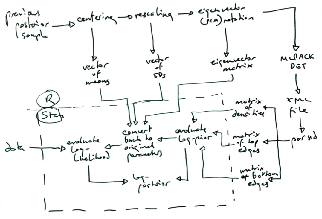
The flowchart below might help to clarify how the objects are created and passed around.
Bayesian windowing and moving weighted averages for streaming data and data drift
In theory, we can use Bayesian updating to get statistical inference not just on accumulating data but also on windows of time. I suspect that the value of Bayesian updating lies mainly in rapidly arriving data (when Big Data people talk about the n Vs, where n is a number unrelated to reality, they usually mention Velocity; voilà!). In that case, there is little point to inference at all once you have accumulated several billion observations. But it is important if you want a moving window of data.
Akidau provides a simple overview of principles here.
If you have fixed windows (see Akidau's figure 8), then each batch of data is in one window. Each window updates the previous ones by taking their posterior and using it as its own prior. If you want to remove an old window, you get its posterior from the archive and subtract its kudzu log-density from your log-prior at each sampling algorithm iteration. But then you have also removed the original a priori priors, and so you should add them back in. However, this adding and then subtracting and then adding accumulates distortion.
So, I think in most cases it will be better to have parallel sequences of updates rather than a single one that has to have p[oste]riors subtracted as well as added. Suppose you are adding new taxi journeys to your model every day. Each window is one day, and you want analyses to be based only on the previous week. It is 7 Jan. I accumulate 1 Jan to 7 Jan in one updated model, and in parallel, 2 Jan to 7 Jan, 3 Jan to 7 Jan, and so on. The final one only has one batch of data in it, 7 Jan. My inferences are based on the full set of weekly updates, which is 1 Jan to 7 Jan. Now, 8 Jan's data arrive. I discard the 1 Jan to 7 Jan analysis, add 8 Jan to all the others, create a new set of updates containing only 8 Jan for now, and use the 2 Jan to 8 Jan set for inference. I need only hire more server cores to run more sequences in parallel.
With sliding windows (see Akidau's Figure 8), the collection of parallel updates wil be governed by the overlap between the windows as well as their length.
We could also apply a weighted window, to reduce the influence of old data. This is analogous to the evergreen exponentially weighted moving average. It would simply be implemented by adding a (negative) log-scaling factor to the kudzu priors. As they got older, they would be suppressed by ever more negative log-scaling factors. However, there is to my knowledge no statistical theory out there about such a weighted posterior, and this should be developed before practical application.
Extended material from the 2021 IJCEE paper
This is where you can find the code and extra graphics from the paper "Non-parametric Bayesian updating and windowing with kernel density and the kudzu algorithm", International Journal of Computational Economics and Econometrics (2022); 12(4): 405-28. doi: 10.1504/IJCEE.2022.10044152 . This paper is available online from the publisher or you can read the post-print here.
Abstract
The concept of "updating" parameter estimates and predictions as more data arrive is an important attraction for people adopting Bayesian methods, and essential in big data settings. Implementation via the hyperparameters of a joint prior distribution is challenging. This paper considers non-parametric updating, using a previous posterior sample as a new prior sample. Streaming data can be analysed in a moving window of time by subtracting old posterior sample(s) with appropriate weights. We evaluate three forms of kernel density, a sampling importance resampling implementation, and a novel algorithm called kudzu, which smooths density estimation trees. Methods are tested for distortion of illustrative prior distributions, long-run performance in a low-dimensional simulation study, and feasibility with a realistically large and fast dataset of taxi journeys. Kernel estimation appears to be useful in low-dimensional problems, and kudzu in high-dimensional problems, but careful tuning and monitoring is required. Areas for further research are outlined.
Prior-only analysis
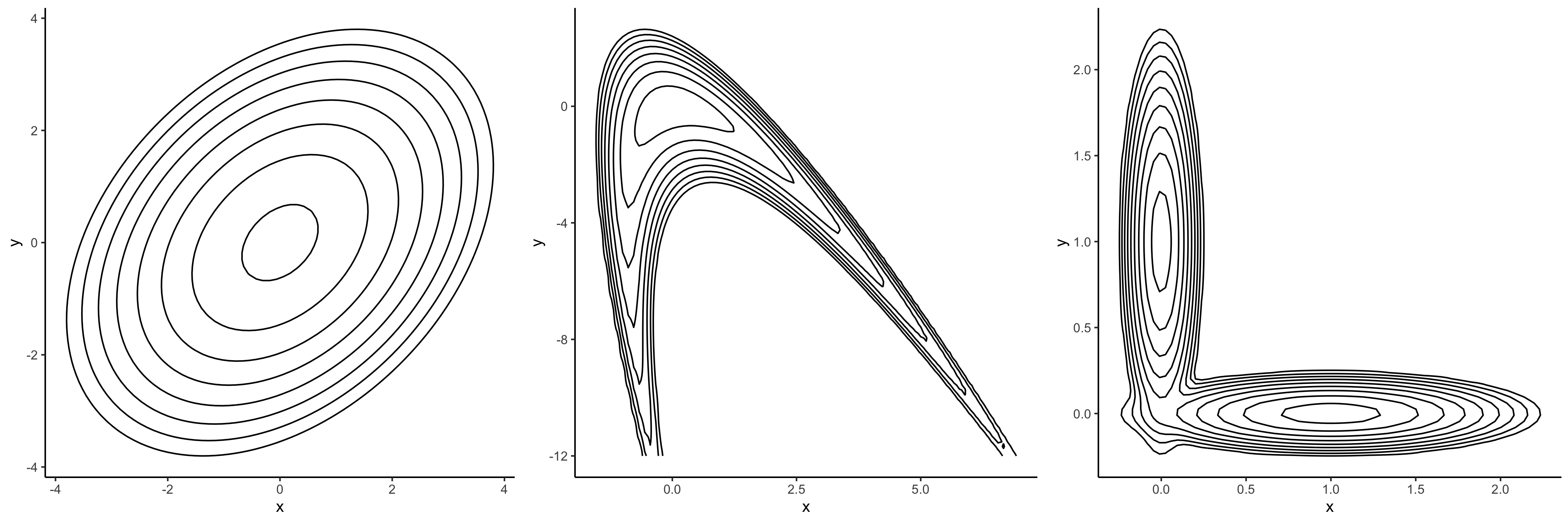
I applied the various methods to samples from these three illustrative two-dimensional prior distributions. These scatterplots of kudzu posteriors under different bandwidths (sigma tuning parameters) for the lasso prior do not appear in the paper.
The kernel and SIR methods are applied in this R file (along with functions for the three prior log-densities and random number generators), and the kudzu algorithm in this R file.
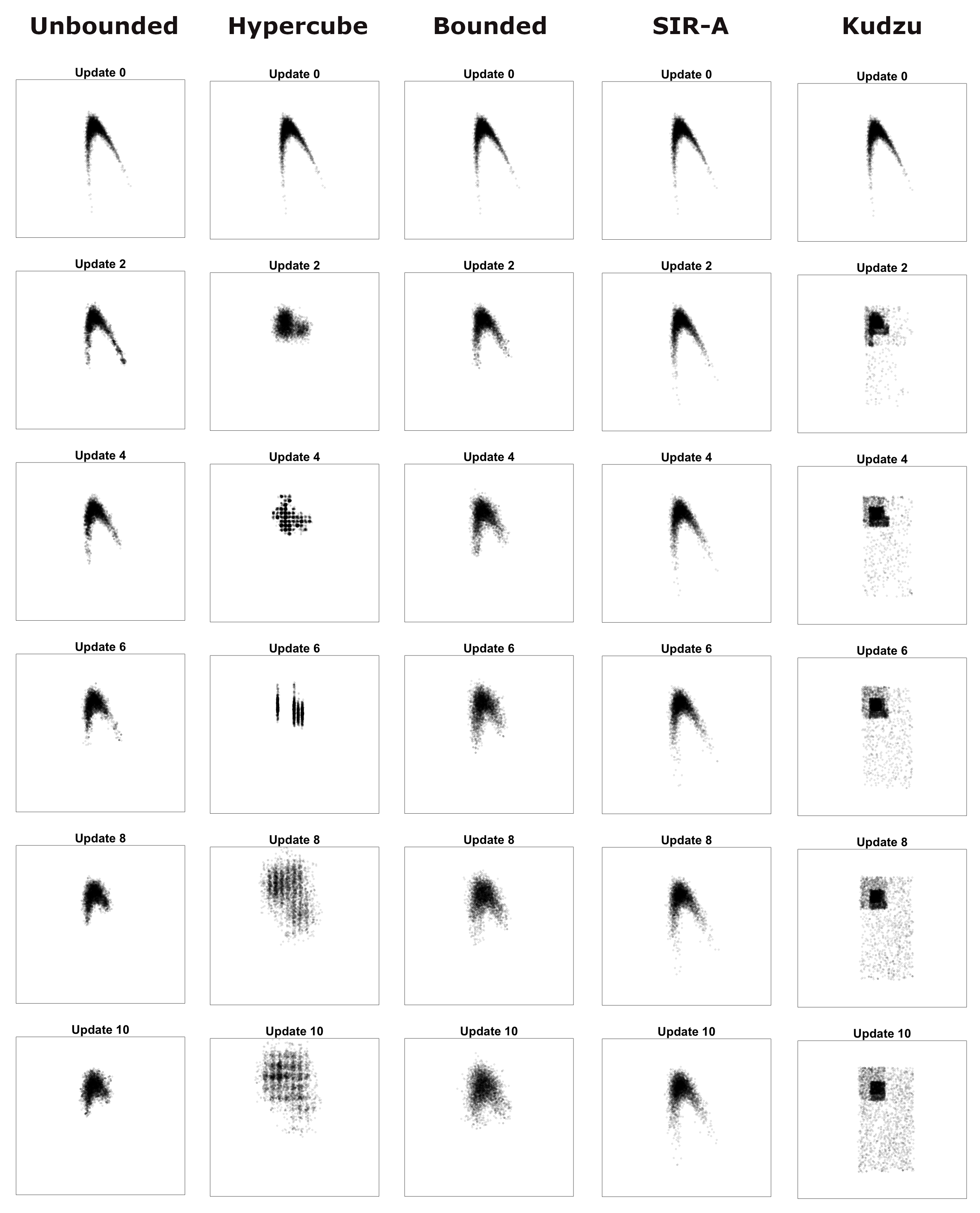
Some of the most interesting output is in these scatterplots of successive posteriors, as we keep updating repeatedly, for every combination of method and distribution (only one of these made it into the paper).
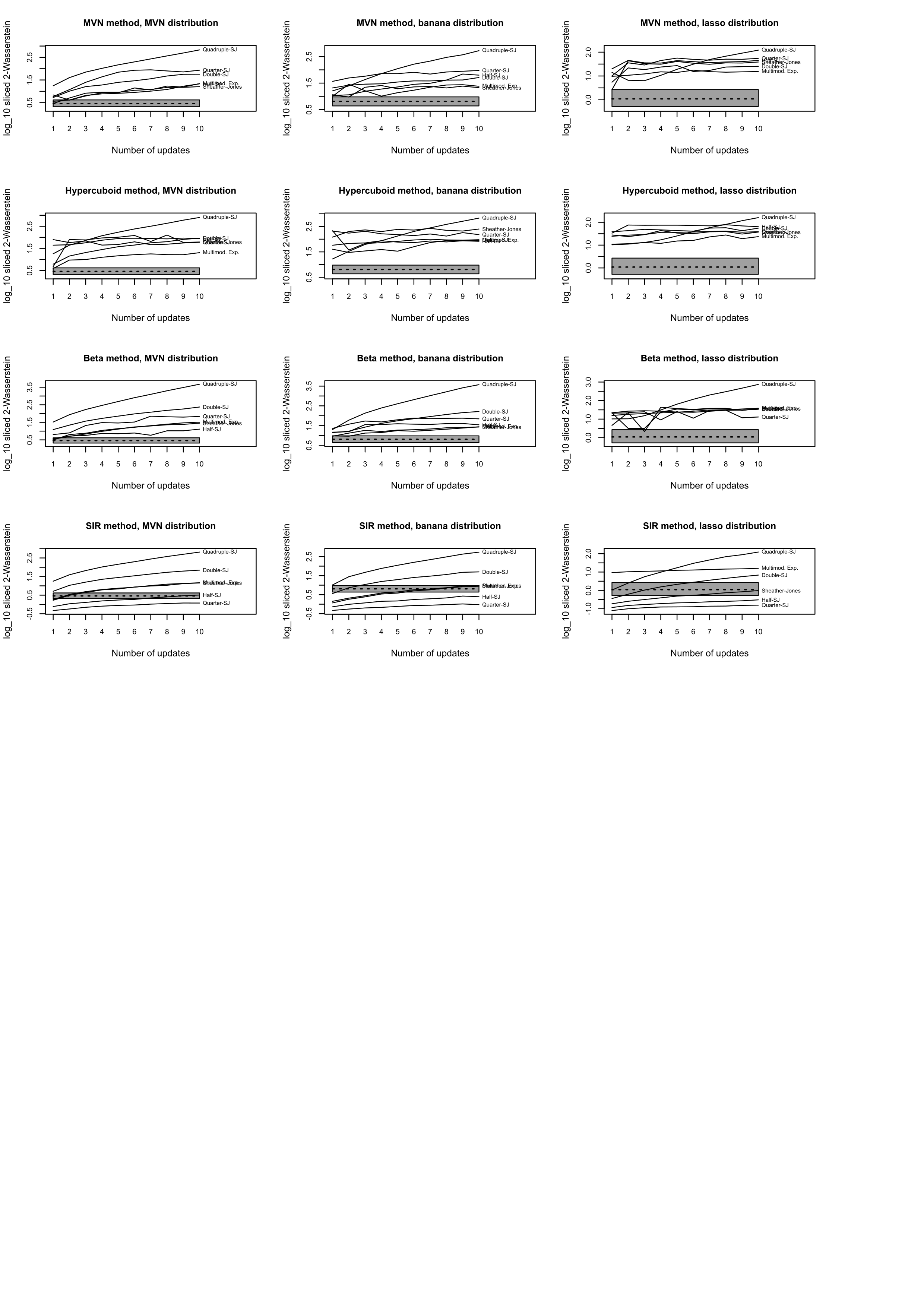
I also summarised distortion using the 2-sliced Wasserstein distance in this R script, then I got the sampling distribution of these Wassersteins under a null hypothesis of pure random sampling thus, and plotted them thus, leading to this image, which was alluded to in the paper, but not printed. You might notice from this that I had parallel folders for the various kudzu bandwidths as proportionate to Sheather-Jones.
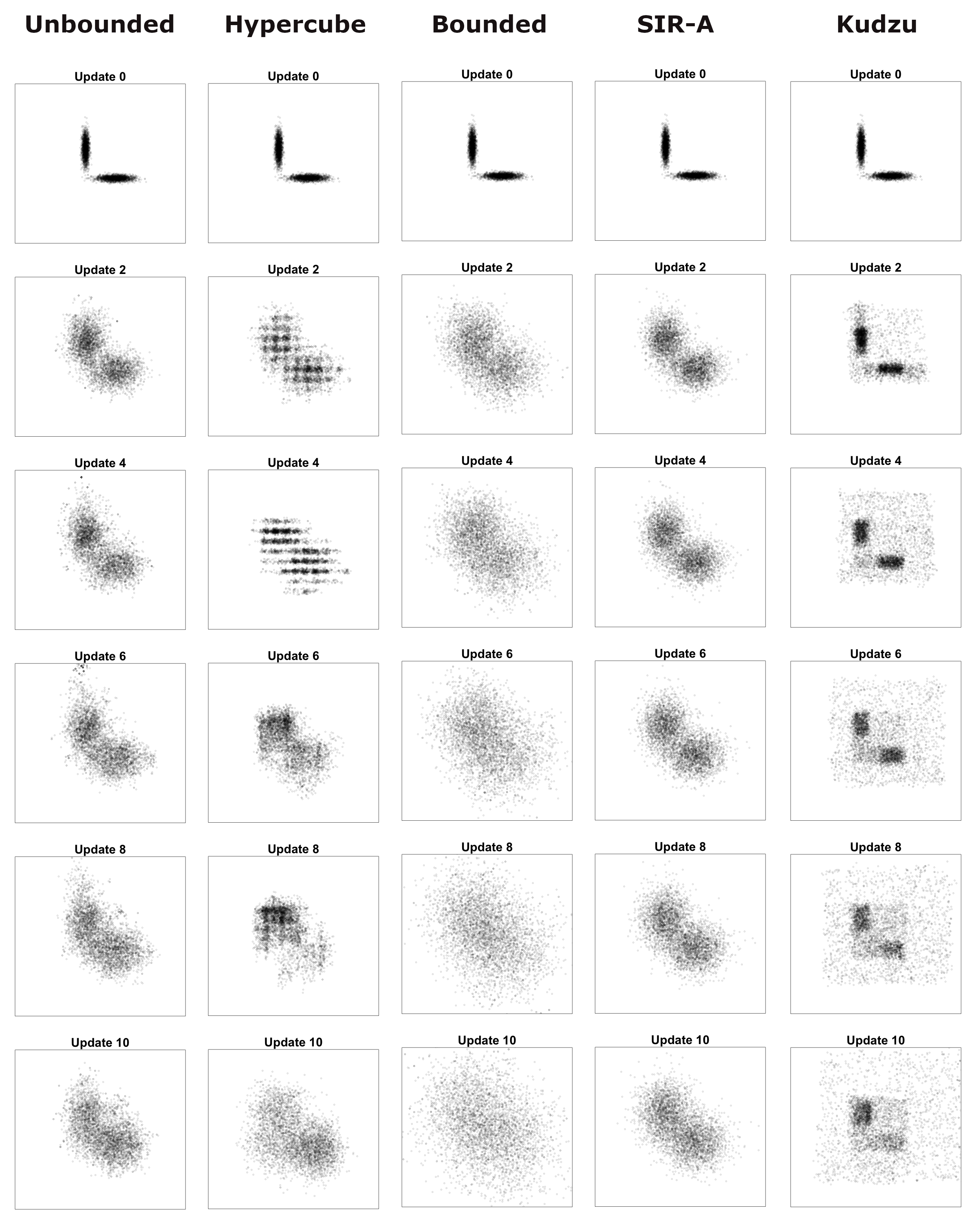
LASSO prior, repeatedly updated without likelihood, by all the methods - click to enlarge. Compare with the banana distribution and the bivariate normal.
Simulation study
I simulated data for a logistic regression model with three parameters, and ran them through ten updates of each of the methods (except kudzu). This ran in a cloud facility virtual machine with 16 cores, so that four instances of R run in parallel, each running its own simulations in folders instance1, instance2, instance3, instance4. This R script executes one of the instances for the kernel methods, while this R script does the same for SIR.
This R script collects simulation study outputs together. The first 30 updates are shown, for each method and each parameter, in this zip file of the Craft charts. They were generated by this R script. The bold curve in each panel is the all-data posterior, which acts as ground truth. The successive posterior means across all simulations are shown in these line charts.
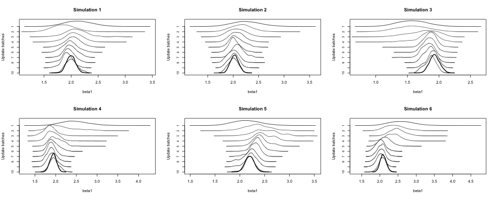
A Craft chart is named after Harold Craft, an astronomer who used a plotter to visualise periodic signals from the first known pulsar. In line with Stigler's Law of Eponymy, these are generally known as Joy Division charts, joyplots, ridgeline plots, &c &c. This zoomed-in section appeared in the paper. The first update's posterior is at the top of each panel, and subsequent updates lead to posteriors moving downward. The bold curve is the all-data (ground truth) posterior.
Feasibility case study: New York taxis
To test out SIR-A and kudzu on a realistically sized problem, I used the first seven days from the 2013 New York yellow taxi dataset, which was originally obtained and shared by Chris Whong. You don't have to download those files to reproduce my analyses; I offer a tidier format below.
My first step is to process each day's "trip file" and "fare file" into a single "taxi data" file. There are the usual GPS errors, for example, and some storage-hogging variables that are discarded after merging. This is the R script for making the taxi data files. But if you want the seven taxi data files, you can grab this zip file (32MB).
Then, I used this data2mats function in R, which will transform a taxi data file in CSV format into a neat collection of R matrices and vectors. This is the data for a given day.
The initial prior is a sample of 210,000 journeys (30,000 from each day). The R code that follows grabs this from the SIR output list, so you can use this to run a reproducible analysis with the same pump-priming prior sample that I used.
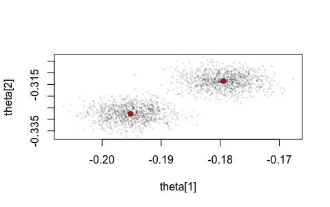
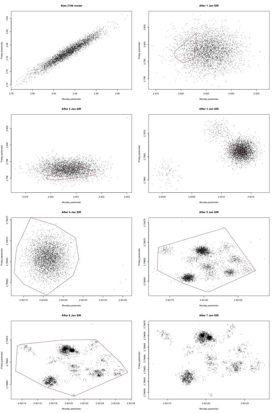
The SIR-A analysis (including data prep) is in this R script (there is no Stan involved for SIR). The output is all in one .rds file. The issue of degeneracy is illustrated by this scatterplot of proposed parameter values from SIR-A, looking at two parameters. The red dots are prior draws and we can see that SIR-A is just samping around them according to the kernel. The kernels overlap marginally but not jointly. Another example is in this set of scatterplots looking at the parameters for Monday and Friday over successive updates. The red polygons are convex hulls of the next p[oste]rior. In this case, degeneracy is not obvious (multimodal) until the likelihood curvature has become comparable to the prior curvature, after a few days.
This R script runs kudzu updates on the taxi data. The Stan models are given separately for prior plus likelihood and for prior only.
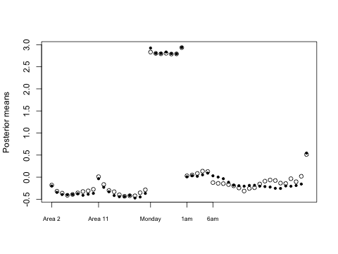
The p[oste]rior means after the n=210,000 pump-priming and after the 1 Jan kudzu update are shown together in this dotplot. The means after pump-priming are hollow circles and those after 1 Jan kudzu are solid black circles. The parameters are in this order:
- nine rectangular regions west of 5th avenue, from downtown to uptown, ending at 110th Street; the most southwesterly is omitted as baseline
- ten rectangular regions east of 5th avenue, from downtown to uptown, ending at 110th Street
- seven days from Monday to Sunday; because none is omitted as baseline, these function as intercept terms
- 23 hours from [01:00, 012:00) to [23:00, 00:00); the first hour [00:00, 01:00) is omitted as a baseline
- the residual standard deviation
The following differences are notable and can be explained to give some reassurance that the update makes sense. Yellow cabs usually have higher fares from midnight to 5:59 by NYC regulations, but this does not apply on 1 January, a public holiday. So, when 1 Jan (n=316,446) is added (so to speak) to the pump-priming (n=210,000 equally drawn from all seven days), we see the drop in fares at 06:00 greatly attenuated, likewise the bump in fares for an evening rush-hour. The Monday intercept term changes somewhat while the other days do not (modulo Monte Carlo error).
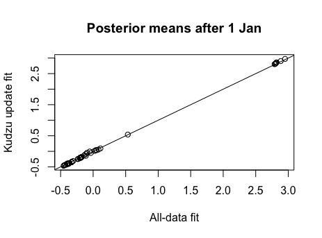
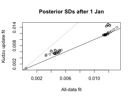
The posterior means after 1 Jan are compared to the prior means here (and they look almost identical), while the SDs are compared here (and they look inflated; the dotted line is double inflation). Succcessive updates don't get much worse, and the inflation is not monotonic over updates, so it may be the early updates that are problematic. Marginal variance inflation is one of the outstanding challenges in appying kudzu effectively. There is much scope for experimentation with adaptive approaches to bandwidth specification and delta-translation.
The effect of bandwidth on posterior variance and covariance is investigated in this R script. Some examples of graphical consideration of the kudzu bandwidth (sigma tuning parameter) are shown in these outputs. We can see when chains diverge because there is not enough gradient within a leaf to guarantee that the chain can escape (sigma=0.008 is too small).
The all-data analyses, which I ran for alternate days, is given in this R script. Posterior stats are compared in this R script.
Further research ideas
More evaluation of kudzu / SIR updating
I have examined kudzu in a mostly if not wholly convex posterior problem, up to p=50. We need to extend that into higher dimensions and trickier posteriors.
My heuristic approach to delta-translation is probably OK with unimodal, convex p[oste]riors. But we need something more flexible. The challenge is that a leaf might adjoin, on the same face, leaves that have a mixture of higher and lower densities than itself. Move towards the higher one and you might inflate variance into the lower one. Move away from the lower one and you might leave a canyon (gully? donga?) between the current leaf and the higher one, which could cause non-convergence, reduced stepsize, all your favourite problems.
SIR-A was tested at p=50 in the IJCEE paper and it flopped badly with degeneracy. However, when it works it is hi-fi and super-fast. We should examine combinations of kudzu and SIR, perhaps kudzu at first and then SIR when the likelihood curvature is greatly exceeded by the prior curvature, and also look at SIR-B.
Not every streaming data problem can have a skilled Bayesian computational statistician watching it 24/7. Perhaps there are some useful approaches for automatically detecting and flagging up SIR degeneracy, such as loss of correlation in the posteriors, multimodality, or posterior standard deviations close to the kernel bandwidths. Similarly, we need automatic monitoring tools for kudzu bandwidths.
I have only tried a crude form of local oversampling for SIR-B, a hypercuboid defined by maximum likelihood estimation. As p rises, the proportion of such a hypercuboid occupied by a hyperellipse (as an example of region where a convex likelihood function exceeds some value) drops rapidly. If we could find the manifold defining such a threshold in the likelihood and locally oversample within that, SIR-B could be truly scalable to high-p. The computational cost of the manifold hunt matters, of course. Of the options that come to mind, I am most interested in:
- SIR-cholesky-B: under an assumption of multivariate normality, or at least convexity, rotate and scale the likelihood so that some off-the-shelf hyperellipsoid could be used
- SIR-hulls-B: find hulls (not necessarily convex though), and locally oversample within them; Ludkin's Hug-and-Hop algorithm comes to mind here
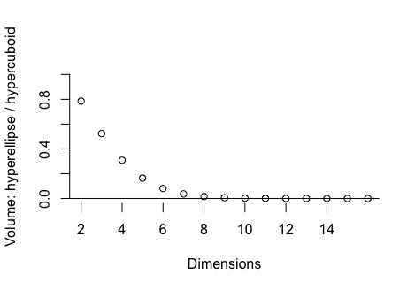
The proportion of hypercuboid volume occupied by a hyperellipse that only just touches the faces of the hypercuboid at two points on either end of each of its axes, as a function of the number of dimensions. This is indicative of the proportion of SIR-B draws that would hit a convex likelihood if drawn from a uniform distribution over the hypercuboid.
More methodology
There are some potential improvements to kudzu, which I am investigating at present (2023):
- ensembles of kudzu, starting with bootstrap aggregation, then extending to boosting and MCMC in the Lie algebra of rotations in p-dimensional space (with reference to projection pursuit)
- asymmetric kudzu, with different sigmas on either side
- formulas to find reasonable plug-in deltas and sigmas, including in the asymmetric case
- assess the potential speed-up versus distortion from approximate (shorter series expansion) of the exponential function
Software development
I am currently (2023) working on R and Stata functionality to:
- fit (and prune) DETs given a sample
- return an estimated piecewise constant density given a new vector and a DET
- return an estimated kudzu density given a new vector, kudzu deltas and sigmas, and either a DET or a user-specified histogram (such as one creates in expert prior elicitation)
- return a marginal or a conditional kudzu density given the above
- efficiently generate pseudo-random numbers from a given kudzu distribution
- return cumulative probabilities given quantiles and a kudzu distribution — or vice versa
- convert my kudzu/DET output to a common object type in R such as from the 'tree' package
I am planning to present these, along with the current methodological work above, at various conferences in 2024.